In a previous post we talked about the first way to estimate a kinship matrix, which is through pedigree. In this post we will cover how to do it with genomic data.
This process is described in detail in the methods session of Proferssor Yang Jian’s landmark 2010 NG paper and you use gcta to generate one. Here I am trying to understand it by recreating the process. See this post on more methods on different flavor of GRM.
Step 1: genotype matrix or SNP matrix.
This part is simple. It’s just converting the vcf to a coded matrix where ref/ref is 0, ref/alt is 1 and alt/alt is 2. Note that this is difference from rrBLUP where the convention is {-1/0/1}. See more about genotype denotation in a previous post. It usually has n rows (number of sample) and m columns (m variants or SNPs).
Step 2: scaling of the genotype matrix.
This genotype matrix is then scaled column-wise, meaning, each variant is scaled on its own based on its allel frequency in this dataset, with the assumption that each locus/SNP is under Hardy-Weinburd Equilibrium (HWE). You see two assumptions are made here. 1. This dataset is representative of the base population therefore the allele frequencies are also representative. 2. Any assumptions that HWE carries such as an infinite random-mating population.
The scaling of the genotype matrix is to ensure that each variant is treated equally to the total genetic effect iregardless of its allel frequency. Mathematically it is to reach a mean of 0 and variance of 1. If the allele frequency of the the alternative state in variant_i is pi, then we scale by minus the mean, which is (2*pi^2 + 1*2*pi(1-pi) + 0*(1-pi)^2) = 2pi, and divided by the sd (var is 2pq is derived from Var(xij) = E(xij^2) - E(xij)^2). Then {0,1,2} (denoted as xij) will become
(xij - 2pi)/sqrt(2*pi*(1-pi)).
To demonstrate let’s have toy dataset with 5 individuals and 3 causual SNPs to a certain trait.
| xij | SNP1 | SNP2 | SNP3 |
|---|---|---|---|
| Individual 1 | 1 | 1 | 2 |
| Individual 2 | 0 | 1 | 0 |
| Individual 3 | 1 | 0 | 1 |
| Individual 4 | 2 | 0 | 0 |
| Individual 5 | 1 | 0 | 0 |
| SUM | 5 | 2 | 3 |
| pi | 0.5 | 0.2 | 0.3 |
First let’s calculate the pi. p1 = (1+0+1+2+1)/10 = 0.5, p2=0.2 and p3=0.3. If Then use the equation (xij - pi)/sqrt(2*pi*(1-pi)). Here is a snipett of code for this calculation:
scale_geno <- function(fi, geno){
  qq <- -2*fi/sqrt(2*fi*(1-fi))
  Qq <- (1-2*fi)/sqrt(2*fi*(1-fi))
  QQ <- (2-2*fi)/sqrt(2*fi*(1-fi))
  a <- ifelse(geno == 0, qq, ifelse(geno == 1, Qq, QQ))
  return(a)
}
In a table it looks like:
| genotype\pi | 0.5 | 0.2 | 0.3 |
|---|---|---|---|
| qq/0 | -1.41 | -0.71 | -0.93 |
| Qq/1 | 0 | 1.06 | 0.62 |
| QQ/2 | 1.41 | 2.82 | 2.16 |
and the scaled genotype matrix (zij) looks like the following. The sum of each column is 0 so the mean is also 0, and the variance of the whole matrix is 1.1, close to the expectation.
| zij | SNP1 | SNP2 | SNP3 |
|---|---|---|---|
| Indi 1 | 0 | 1.06 | 2.16 |
| Indi 2 | -1.41 | 1.06 | -0.93 |
| Indi 3 | 0 | -0.71 | 0.62 |
| Indi 4 | 1.41 | -0.71 | -0.93 |
| Indi 5 | 0 | -0.71 | -0.93 |
| SUM | 0 | 0 | 0 |
Step 3: turning a genotype matrix (n x m) into a relationship matrix (n x n)
By now, we should be able to have a relationship matrix between these five individuals by doing ZZ’/m(=3). Let’s call it the G matrix and it is 5 X 5 in this case.
| G | Ind1 | Ind2 | Ind3 | Ind4 | Ind5 |
|---|---|---|---|---|---|
| Ind1 | 1.93 | 0.30 | 0.20 | -0.92 | -0.92 |
| Ind2 | 0.30 | 0.70 | -0.44 | -0.63 | 0.04 |
| Ind3 | 0.20 | -0.44 | 0.30 | -0.02 | -0.02 |
| Ind4 | -0.92 | -0.63 | -0.02 | 1.12 | 0.46 |
| Ind5 | -0.92 | 0.04 | -0.02 | 0.46 | 0.46 |
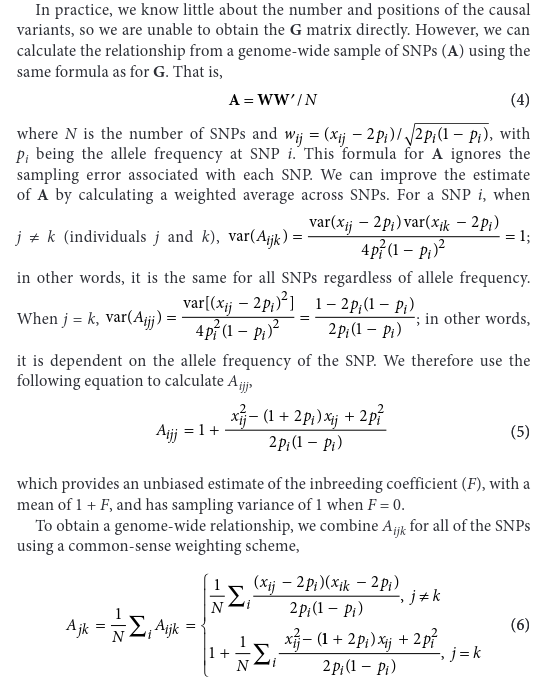
In reality, we know little about where the causual SNPs are. Instead, we will just use all the SNPs, as long as some of them are tightly linked to the actually QTLs. However this assumes that the allele frequency we see in our dataset hold true for the population, which ignores the sampling error associated with each SNP. In order to improve the estimate of G, Yang 2010 proposed a weighted average across all SNPs. In this method, the values on the off-diaganols is the same as ZZ’/m. The only adjustment happens on the diaganols (equation 5 in the image below). Specifically, they are defined as 1+F and F is called inbreeding coefficient. I know how to calculate the inbreeding coefficient when considering one locus, which is 1 - H(O)/H(E), H(O) for observed number of heterozygotes and H(E) for expected number of heterozygotes under HWE. However I do not know how you calculate F when there are multiple loci. The j=k part in Equation 6 sums it up for all the SNPs and return a 1+F for each individual based on Eq. 5, but I do not understand why Eq. 5 is true. They lost me at When j=k, var(Aijj) part. But let’s just use on our small toy dataset for now.
Aijj <- function(p, x){
  f <- (x^2 - (1+2*p)*x + 2*p^2)/2*p*(1-p)
  a <- 1 + f
  return(a)
}
| Aijj | SNP1 | SNP2 | SNP3 | Ajj(mean) |
|---|---|---|---|---|
| Indi 1 | 0.9375 | 0.9744 | 1.1029 | 1.0049 |
| Indi 2 | 1.0625 | 0.9744 | 1.0189 | 1.0186 |
| Indi 3 | 0.9375 | 1.0064 | 0.9559 | 0.9666 |
| Indi 4 | 1.0625 | 1.0064 | 1.0189 | 1.0293 |
| Indi 5 | 0.9375 | 1.0064 | 1.0189 | 0.9876 |
Note that for heterozygotes (1), the number is smaller than 1 (f is negetive) and the homozygote, the number is greater than 1 (f is positive). This matches with our understanding of increasing in homozygosity where in inbreed. The last column is the average over i or across the SNPs. Now we can see that among those 5 individuals, number 3 and 5 are outbreed and the rest are inbreed. But this does not match with intuition. Indi 1 has two hetero site out of 3, why it is above 1? Need to check futher. Assuming this is correct, now we can replace the diaganols with the new calculations.
| A | Ind1 | Ind2 | Ind3 | Ind4 | Ind5 |
|---|---|---|---|---|---|
| Ind1 | 1.00 | 0.30 | 0.20 | -0.92 | -0.92 |
| Ind2 | 0.30 | 1.02 | -0.44 | -0.63 | 0.04 |
| Ind3 | 0.20 | -0.44 | 0.97 | -0.02 | -0.02 |
| Ind4 | -0.92 | -0.63 | -0.02 | 1.03 | 0.46 |
| Ind5 | -0.92 | 0.04 | -0.02 | 0.46 | 0.99 |
We can see that the order changed. Previous from low to high it was 3,5,2,4,1, now it is 3,5,1,2,4. Still something with Indi 1. But the ones on the diaganols are closer to 1 comparing to G.
Currently I am using gcta and then I convert it from bin format to the txt format. gcta offers a snipet of code for the conversion but it did not work for me. Here is my snipet:
read_grm <- function(prefix) {
  # Construct file paths based on the prefix
  grm_bin <- paste0(prefix, ".grm.bin")  # Binary file containing the GRM
  grm_id <- paste0(prefix, ".grm.id")    # File containing IDs (individuals)

  # Step 1: Read the ID file
  grm_ids <- read.table(grm_id, header = FALSE, stringsAsFactors = FALSE)
  colnames(grm_ids) <- c("FID", "IID")

  # Step 2: Read the binary GRM file
  # Read the size of the binary file (each element is stored as a 4-byte float)
  n <- nrow(grm_ids)  # Number of individuals
  grm_data <- readBin(grm_bin, what = "numeric", size = 4, n = n * (n + 1) / 2)

  # Step 3: Reshape the GRM data into a matrix
  # Initialize an empty matrix to store the GRM values
  grm_matrix <- matrix(0, n, n)

  # Fill the matrix from the GRM binary file (which is in lower triangular format)
  index <- 1
  for (i in 1:n) {
    for (j in 1:i) {
      grm_matrix[i, j] <- grm_data[index]
      grm_matrix[j, i] <- grm_data[index]  # Symmetrize the matrix
      index <- index + 1
    }
  }

  # Add row and column names using the IDs
  rownames(grm_matrix) <- grm_ids$IID
  colnames(grm_matrix) <- grm_ids$IID

  # Return the GRM matrix
  return(grm_matrix)
}
Is there R code that takes the genotype matrix and gives the GRM? I am sure I am reinventing the wheel here. Le’t try the A.mat from rrBLUP.
M <- matrix(c(1,1,2,
              0,1,0,
              1,0,1,
              2,0,0,
              1,0,0),5,3)
# rrBLUP decodes in {-1,0,1}
M <- M-1
A <- A.mat(M)
OK we are not done yet!
Now let’s hand calculate the right side of the the methods section of Yang 2010 which is “Unbiased estimate of the relationship at the causal variants and the genetic variance”, or A*.
The result is very different… OK let’s explore more tomorrow. hand calculation vs. gcta bin to txt vs. A.mat.