IBD at allele level
Identity-by-descent, also known as identical-by-descent, is used to describe two homologous alleles that have descended from a common ancester. Homologous here means that they are the same (identical). You can compare two alleles from different individuals or the same diploid individual.
IBS
Identity-by-state, also known as identical-by-state. This concept is relatively simple. It just means that two alleles are homologous, iregardless whether they are IBD. This sounds familiar right? The relationship between IBD and IBS is like the one between orthologs and homologs. IBS is what we see in the current dataset.
There we borrow an illustration from [Powell 2010]((https://www.nature.com/articles/nrg2865) to demonstrate the difference between IDB and IBS.
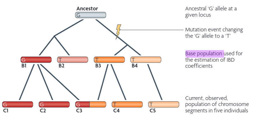
So in this figure, as long as the letter is the same, they are IBS, so all the Gs and all the Ts are IBS respectively. However, you also need to have the same background color to be IBD. For example, C1 and C2 are IBD, B3 and B4 are not IBD, C4 and C5 are not IBD either.
prob(IBD) = F = Inbreeding coefficient
The probability of IBD between two alleles is denoted as F.
How to calculate F for a specific locus? It can be achieved by comparing the observed heterozygosity rate with the expected one under Hardy-Weinberg Equilibrium. We already know that inbreeding, defined as mating between individuals sharing a common parent in their ancestry, is one of reasons for deviation from HWE. If there is only random mating (one of the assumption of HWE), meaning no mating between individuals sharing common ancestry, i.e. no inbreeding, there would be no IBD (F=0), and we all know that the frequency of genotypes would look like: GG = p^2, GT = 2pq, TT = q^2. In this case, the homologous alleles (GG or TT) are actually from different ancesters; they just happen to be the same. OK now you see how this might contradict with the coalescence theory where there is only one common ancester (they did not just HAPPEN to be the same!) but it is in the other post.
Now let’s add inbreeding into the picture. Because of inbreeding, some of the homologous alleles are actually from the same ancester (IBD), and we already denoted this probability as F. For this portion (F), since they are IBD, they can only be GG or TT, therefore their relative frequency for GG/GT/TT is p/0/q. For the rest (1-F) that are still under HWE, the relative frequency for GG/GT/TT is still p^2/2pq/q^2. So in the current population, the genotype frequency would be:
- GG: F * p + (1-F) * p^2 = p^2 + pqF
- GT: (1-F) * 2pq = 2pq - 2pqF
- TT: F * q + (1-F) * q^2 = q^2 + pqF
Notice how pqF is effectively “taken” from the heterozygotes and added to each homozygote class.
If the two alleles are in the same diploid individual then F is also called the inbreeding coefficient of the individual at this locus.
If the two alleles are in different individuals, F can be used to calculate the numerator relationship between them as in a A matrix. The co-ancestry of two diploid individuals is the average of the four F values from the 4 possible comparisons between each pair of alleles (2 choose 1 * 2 choose 1); their numerator relationship, or the off-diagonals on their A matrix, is twice their co-ancestry. Note that this is slightly different from what we did in the A matrix post, where it was defined as a_ind1,ind2=0.5(aind1,sire2 + aind1,dam2), where the numerator relationship is the average of ind1 ‘s relationship with ind 2’s parents. Using the same rationale, the numerator relationship of a diploid individual and itself (diagonals of A matrix) would be (1 + 1 + F + F)/4 * 2 = 1 + F, given the probability of IBD of the same allele is 1.
In Speed and Balding 2015, it is defined as the “phenomenon whereby two individuals share a genomic region as a result of inheritance from a recent common ancester, where ‘recent’ can mean from an ancestor in a given pedigree, or with on intervening mutations event or with no intervening recombination event.”
” is tightly linked to “Traditional measures of relatedness, which are based on probabilities of IBD from common ancestors within a pedigree, depend on the choice of pedigree”. If the pedigree is known, the expected IBD is [A matrix].
IBD at segment level
“In this definition of ‘chromosome segment IBD’ there is no need for a base population.”
However unfortunately there is no consistant definition of IBD probabilities without pedigree.
However when the pedigree is unknown, IBD relationships can only be inferred from the population at speculation, and unfortunately there is no consist
In another review paper, Powell 2010 defined it as “alleles that are descended from a common ancestor in a base population”. You can see the two definitions are slightly different. The former uses “genomic region” as the unit whereas the latter uses “alleles”. Alleles are versions of genes, where as “genomic region” can be non-genic, also can be of any length, so the former is more generic. Also, the latter emphasized on the concept of “base population”. The probability of IBD is sometimes referred to as F, and it “has to be defined with respect to a base (reference) population; that is, the two alleles are descended from the same ancestral allele in the base population.” Why so? As you can imaging, if an allele is very rare in the base population, then the possibility of IBD is very high. On the contrary, if an allele is very prominant in the base population, two individuals having the same allele could be due to chance. See another post on how to determine the base population.
“If the two alleles are in the same diploid individual then F is the inbreeding coefficient of the individual at this locus.” See more on how IC is calculated in this post.
IBS is usually used to calculate the G matrix with unknown pedigree. As you can see this can lead to erroneous inference because a consistent base population is not used.
Note that this relationship is usually considered within the same generation, not crossing generations. Another thing to note in this figure is that the base population used for the estimation of IBD coefficients should be B1, B2, B3 and B4, not the current C1 to C5. This is why you need to specify the founders or any know pedigree info in the .fam file. I wonder whether gcta takes this info? I tried but it does not :(
What plink offers
PLINK provides tools to calculate genetic similarity between individuals using IBS and Hamming distance. IBS measures the proportion of alleles shared between two individuals across all markers. It ranges from 0 (no alleles shared) to 1 (all alleles shared). Hamming distance measure the mismatches between two individuals, therefore they are inversely related, and it is specified as [‘1-ibs’]. You can choose based on whether you’d like a similarity matrix (ibs) or distance matrix (1-ibs).
This is an option called flat-missing. The manual reads:
“Missingness correction
When missing calls are present, PLINK 1.9 defaults to dividing each observed genomic distance by (1-<sum of missing variants’ average contribution to distance>). If MAF is nearly independent of missingness, this treatment is more accurate than the usual flat (1-
But how do I know if MAF is dependent of missingness or not in my data? In this case you can investigate their relationship in your own data by generating those two stats.
plink --bfile data --mising --out stats
plink --bfile data --freq --out stats
Then you can calculate the correlation of the F_miss column in the .lmiss file and the MAF column in the .frq file. If it is significantly greater than 0, there might be a correlation. In my case it is amost 0.15 therefore I should turn on the flat-missing option. Then the cmd looks like:
plink --bfile plink_data --distance ibs flat-missing --out ibs_distance
These metrics are useful for understanding relatedness, population structure, and data quality.
from HWE to F
Equation 1 shows how to adjust the usual Hardy–Weinberg genotype frequencies to account for inbreeding. Suppose you have two alleles, G and T, with frequencies (q) and (p = 1 - q) in the base population. Then the genotype probabilities in a population with inbreeding coefficient (F) become:
[
\begin{aligned}
P(\text{GG}) &= q^2 + pqF,
P(\text{GT}) &= 2pq(1 - F),
P(\text{TT}) &= p^2 + pqF.
\end{aligned}
]
Below is a step-by-step explanation of why this formula makes sense.
1. No Inbreeding ((F = 0)): Hardy–Weinberg
Recall that in a random-mating (non-inbred) population under Hardy–Weinberg equilibrium, the genotype frequencies are:
[ P(\text{GG}) = q^2, \quad P(\text{GT}) = 2pq, \quad P(\text{TT}) = p^2. ]
If we set (F = 0) in Equation 1, it simplifies back to the usual (q^2,\, 2pq,\, p^2). This confirms that the formula is consistent with standard Hardy–Weinberg when there is no inbreeding.
2. Complete Inbreeding ((F = 1))
If (F = 1), every individual is completely autozygous (homozygous by descent). Then the probability of being homozygous for G is (q), and for T is (p). The formula becomes:
[ P(\text{GG}) = q, \quad P(\text{GT}) = 0, \quad P(\text{TT}) = p, ]
meaning no heterozygotes at all (all individuals are homozygous). This matches the extreme case of complete inbreeding.
3. Partial Inbreeding ((0 < F < 1))
When (F) is between 0 and 1, a fraction (F) of the population is “autozygous” (forced to be homozygous), while the remaining fraction ((1-F)) follows the usual Hardy–Weinberg proportions. Algebraically, you can think of it as:
- With probability ((1-F)), an individual has genotype frequencies (q^2 : 2pq : p^2).
- With probability (F), the individual is homozygous, and the chance of G vs. T is (q) vs. (p).
Putting these together:
- GG: ((1-F)\,q^2 + F\,q = q^2 + pqF)
- GT: ((1-F)\,(2pq) = 2pq(1-F))
- TT: ((1-F)\,p^2 + F\,p = p^2 + pqF)
Notice how (pqF) is effectively “taken” from the heterozygotes and added to each homozygote class.
Why This Matters
- Increased Homozygosity:
As (F) increases from 0 to 1, you see fewer heterozygotes ( (2pq(1-F))) and more homozygotes ( (q^2 + pqF \text{ or } p^2 + pqF)). - Interpreting (F):
The inbreeding coefficient (F) quantifies the probability that the two alleles an individual carries are identical by descent. Higher (F) means a greater chance of inheriting the same ancestral allele on both chromosomes, hence more homozygosity.
In Summary
Equation 1: [ \text{GG: } q^2 + pqF, \quad \text{GT: } 2pq(1-F), \quad \text{TT: } p^2 + pqF ] is the standard way to incorporate inbreeding into genotype frequencies. It smoothly transitions between:
- Hardy–Weinberg proportions when (F = 0).
- Complete homozygosity when (F = 1).
- Intermediate levels of homozygosity for (0 < F < 1).
Thus, the formula neatly captures how inbreeding inflates homozygote frequencies and deflates heterozygotes relative to the baseline Hardy–Weinberg expectation.